Interpolation is a very useful technique for extracting data when the available information does not come in a continuous form.
From a non-technical point of view, any inference or decision process (sometimes subconsciously) is based on a kind of interpolation or best fitting or regression of the available informations. We as people are normally quite good at generalising (often too fast) from the little amount of information that we have about other people, situations, or even numerical data. This is possible because our brain can recognise patterns and see trends in any kind of data. However, technically speaking, interpolation is more that just finding a trend.
Technically, we are often given a discrete set of data corresponding to a certain function which is known at specific points, or nodes (for example, we have made an experiment for specific input values and measured the outputs corresponding to that input), and is otherwise unknown. In principle this is a multi-dimensional problem, and the interpolating hyper-surface will give an idea of the missing information. In fact, even if it is true that such a hyper-surface can always be numerically constructed, however the uniqueness issue remains. Given the same input data, many different constructions can be engineered, all satisfying to various -more or less realistic- criteria, and all passing through the same input points.
This non-uniqueness property is due to the overwhelming amount of freedom that one has when setting up an interpolation procedure. On one side, the interpolation function could be almost anything, on the other side the only necessary constraint is that the function pass through the nodes. The latter sounds like a very strong constraints, but in reality it is not, since it is not enough to fix many parameter that are otherwise undetermined and free. What we can do is: we can play with additional constraints that make our solution look good. By doing that we can steer the outcome to have certain properties. We will see now how this works in practice by considering the one-dimensional case.
The function is known only at the specific input values, and is otherwise unknown.
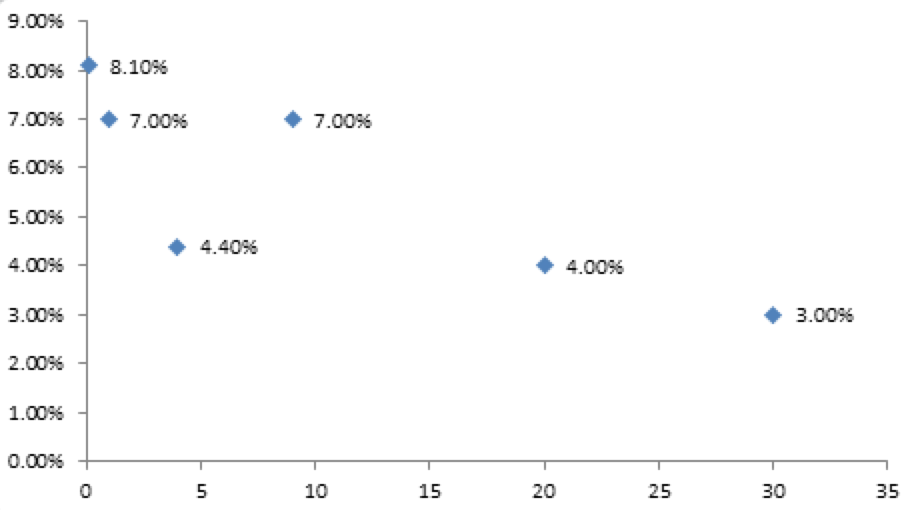
In the one-dimensional case, the solution that we are looking for is a one-dimensional function f(x). The function is known only at the specific input values of the x variable, and is otherwise unknown. For example, in this plot some values of an unknown function f are shown in correspondence to the input x variable equal to 0.1, 1, 4, 9, 10, 20, 30 (we don't need to concern ourself about what on the x and y axis is). The question is now: can we construct a curve that passes through all the points, and if so how? The answer to this question is yes, and there are many ways to do it.
Typical features of the interpolating function that we can play with when we perform an interpolation procedure are the following:
- Passing through the points. This is always guaranteed by definition on interpolation.
- Continuity. It is always guaranteed by construction.
- Smoothness. Depending an the method used in the interpolation, the interpolating function can be more or less smooth at the node points (it is of course always smooth away from the nodes). For instance, in linear interpolation, it is not differentiable by definition, since the sloop changes abruptly at the node points, while in spline interpolation differentiability is achieved by requiring proper boundary conditions for the derivatives at the nodes.
- Piecewise. The interpolation function is typically defined piecewise. This means that the function is determined by using only a few of the data points (typically two or three consecutive ones) plus enforcing additional constraints at the boundaries of each interval.
- Zig zag behaviour. This strongly depends on the chosen method. Some methods (e.g. the polynomial interpolations) manifest a strong oscillating -and unrealistic- behaviour between consecutive data points; others instead (e.g. the monotone preserving cubic spline) use an additional constraints to guarantee some degree of monotonicity in the solution.
There are many methods available in the mathematical literature. Generically speaking, we have a few categories. The simplest method is linear interpolation, where one simply connects any two consecutive points with a straight line. As a result, the curve will show non-differentiable spikes., which is not always what we are looking for. In order to account for such an unwanted feature, there are several polynomial-like interpolation techniques (including the splines), where a polynomial curve is drawn through consecutive points. The degree of smoothness is now connected to the choice of how many derivatives we want to be constrained to be continuous. The drawback is however a strong -and probably unrealistic- oscillating behaviour between the node points, which is not an intrinsic feature of the true function but a spurious effect created by the chosen interpolation method. Finally, in order to take this oscillations into account, some algorithms have been developed that enforce monotonicity of the interpolating function, in such a way that the trend of the curve follows the trend of the data points.
What about finance?
In finance, interpolation is used in many places and is at the basis of pricing every financial product. One crucial place where it appears is the yield curve that describes the term structure of interest rates. Such a curve is constructed out of a few data points (the interest rates are typically known only for a discrete set of maturities) and hence it is crucial to find the best interpolation method for the intermediate maturities that does not produce unwanted effects, such as the unrealistic up-down jumps of a polynomial interpolation. Also other important quantities, such as the forward rates, are defined in terms of the first derivative of the yield curve, hence it is important for such a curve to be continuous and differentiable. Moreover forward rates cannot be zero by the arbitrage principle, and that adds a further constraint when testing an interpolating curve.
The latter point has been -and still is- a great source of debate, mainly because almost all the known methods fail this forward-positivity test for some very specific input points. That holds true even with the extensively used cubic splines (e.g the famous Hermite or the monotone preserving splines). In their papers (here and here) Hagan and West have introduced a new interpolation method which is constructed using the forward rates as fundamental variables and is guaranteed to pass the positivity test. The method is an improved method of the row interpolation, where the forward rates are recognised to be constant in each intervals. Besides positivity, it also enforces monotonicity, thus avoiding those unrealistic jumps that plagued a spline-like interpolation. The zero rates are obtained by inverting the forwards. The integral in the calculation of the zero rates makes sure that they will be continuous. It is fair to say that, due to its very origin, the Hagan-West method is only suitable for financial application, and in particular it is relevant in pricing interest rate derivatives. However, we advice everybody to read this paper at least once, both for its technical content and for its relevance on today's pricing models.
What about the forward rates? Are they guaranteed to be continuous?
The answer is no. By working on our financial library, which also implements the Hagan-West interpolation, we bumped into a case where the Hagan-West method does produce discontinuous forward rates. The table represents our input for the zero rates and the plot is the forward curve constructed out of these data. The input data are not at all strange or cooked-up just to make a point, but they are rather standard. That clearly makes the method weaker.
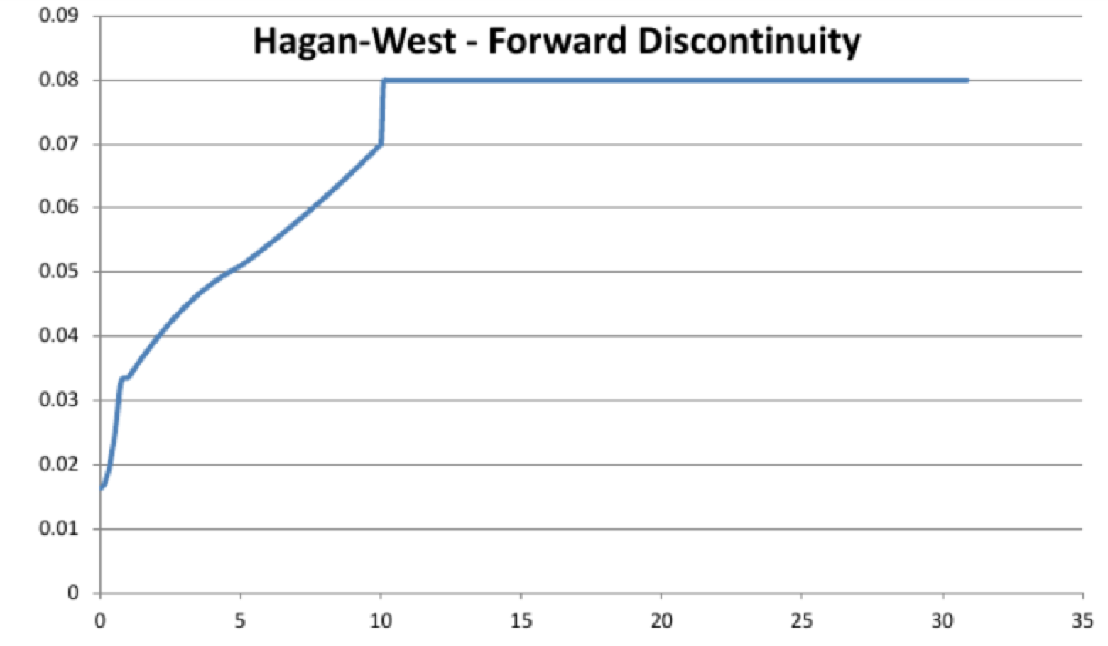
Discontinuity in Hagan West - fwd plot
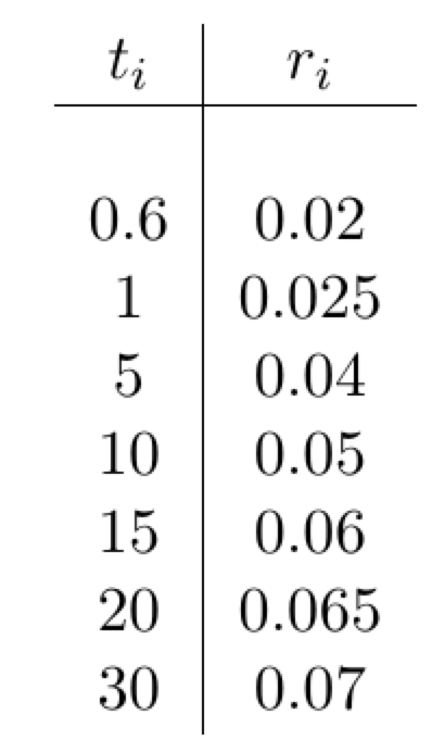
Discontinuity in Hagan West - input table
We discovered this feature of the Hagan-West interpolation method while working on UDFinLib. Later, while doing research to figure out whether this was a real effect or whether we had made a mistake somewhere, we found that this problem with Hagan-West's method was already known to some people (see this), even if the solution that was proposed there does not look fully satisfactory to us, mainly because monotonicity is compromised.
At this point the real question is: there will ever be a perfect method that satisfies to all the constraints (continuity, positivity, differentiability, monotonicity, etc..) of the zero rates and/or the forward rates? So far it seems that there is not a solution that meets all the requirements. But maybe this is only a matter of time. Or is there something conceptual that we are missing?