In this blog we want to demonstrate the power of Octave for doing simulations. Specifically we will take a look at the Black Scholes formula and how fast an option price computed using Monte Carlo simulation will converge to the actual value using the closed-form solution. The idea is to demonstrate how Octave can be used for this kind of simulations. In a previous blog we showed how to created plots, so here will will focus on the simulation only. The mantra when using Octave is "use vectors and matrices". If you can pull that off, your code will be efficient. On the other hand if you need to resort to for-loops, that will slow things down significantly.

Black Scholes Closed-Form

Fist we need to implement the Black Scholes formula in Octave. This is pretty straight forward if you have been working with either Matlab or Octave for a while. We looked here for inspiration and modified the code to make it more compatible with this experiment.

function [C, P]= blackScholes(S,X,r,sigma,T)
    d1 = (log(S/X) + (r + 0.5*sigma^2)*T)/(sigma*sqrt(T));
    d2 = d1 - sigma*sqrt(T);
    N1 = 0.5*(1+erf(d1/sqrt(2)));
    N2 = 0.5*(1+erf(d2/sqrt(2)));
    C = S*N1-X*exp(-r*T)*N2;

    N1 = 0.5*(1+erf(-d1/sqrt(2)));
    N2 = 0.5*(1+erf(-d2/sqrt(2)));
    P = X*exp(-r*T)*N2 - S*N1;
end

The result from this function will give us an absolute "truth" to verify the accuracy of the simulation result. 

Geometric Brownian Motion

We use the geometric Brownian motion for the simulation of the underlying asset. To get the option price from the simulation one:

• uses the MAX function to evaluate the payoff
• discounts to get present value.

In the code below "W" is a vector of size i * step by one filled with random normal variables. This will result in W being a vector (hence the 1) of random numbers depending on i. The index i will be increased using a for-loop so we can see the convergence for each step.

Computation of the present value is done by discounting using the "exp(-r*T)"-term.

  W = randn(i * step,1); 
 
  S_T = S * exp((mu-sigma*sigma*0.5)*T+sigma*sqrt(T)*W);
  C_mc(i) = mean(max(S_T - X, 0))*exp(-r*T);
  P_mc(i) = mean(max(X - S_T, 0))*exp(-r*T);

A complete listing of the code used for filling C_mc and P_mc with call and put values for increasing number of simulations is given in the appendix below. Most of the listing contains the code used to generate the plots presented in the next chapter.

Results

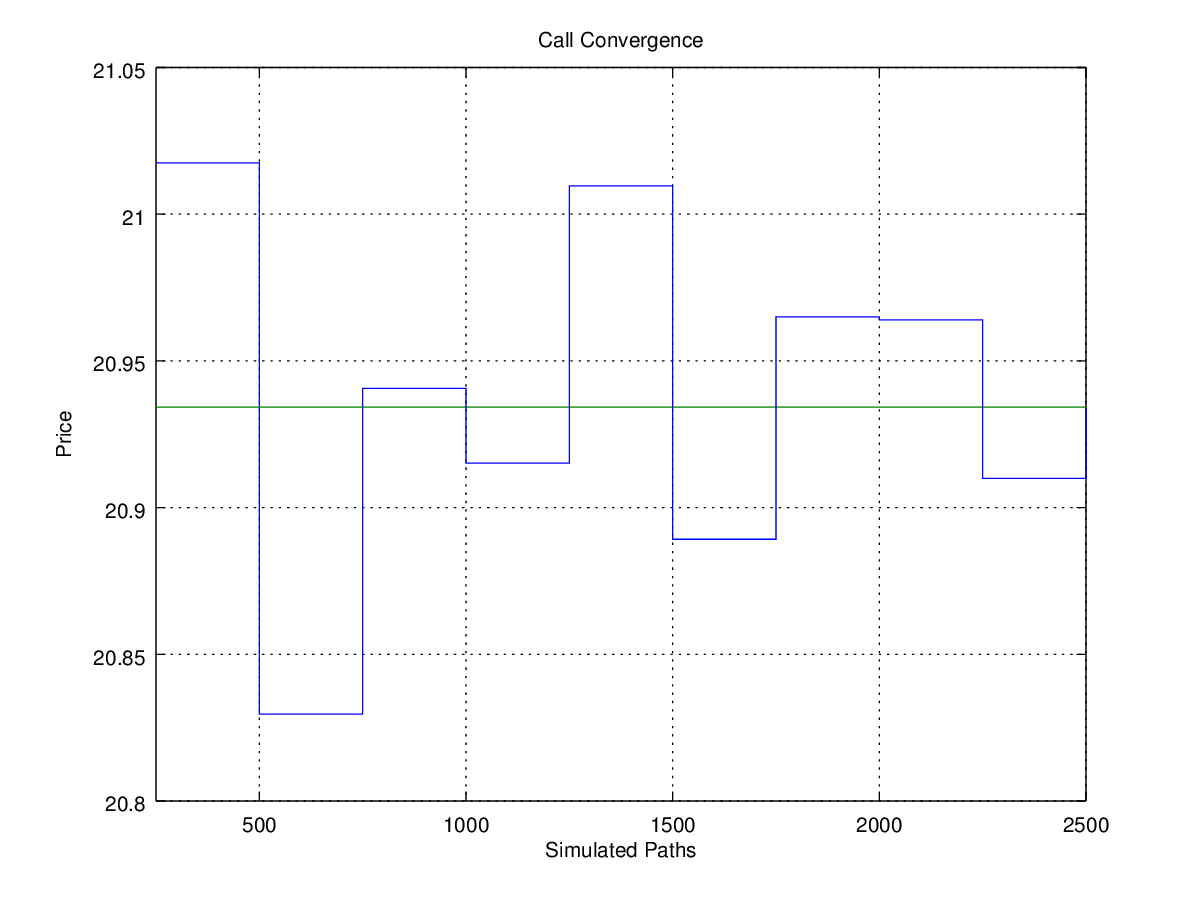
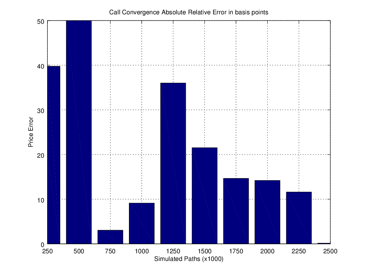
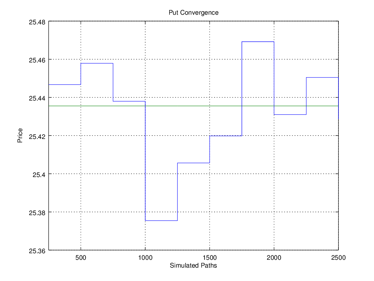
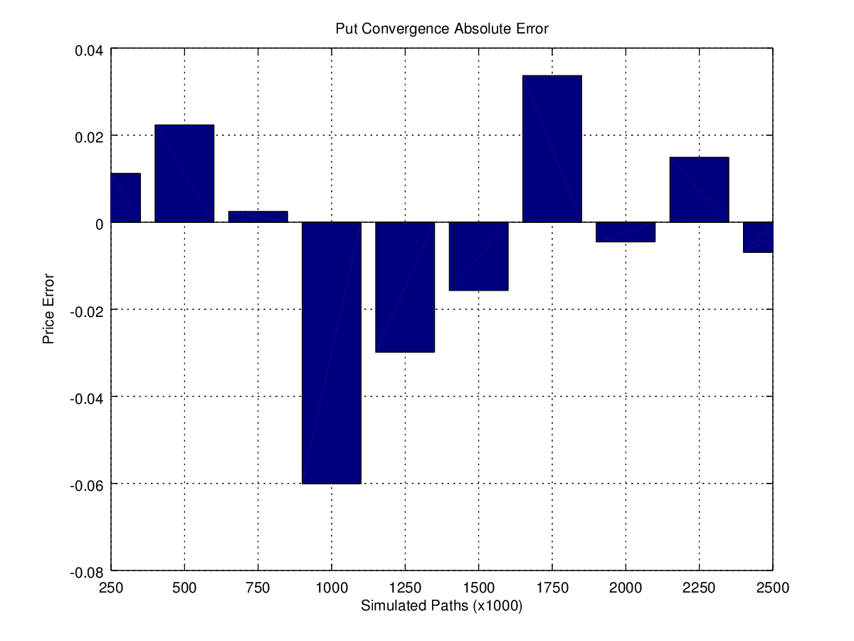
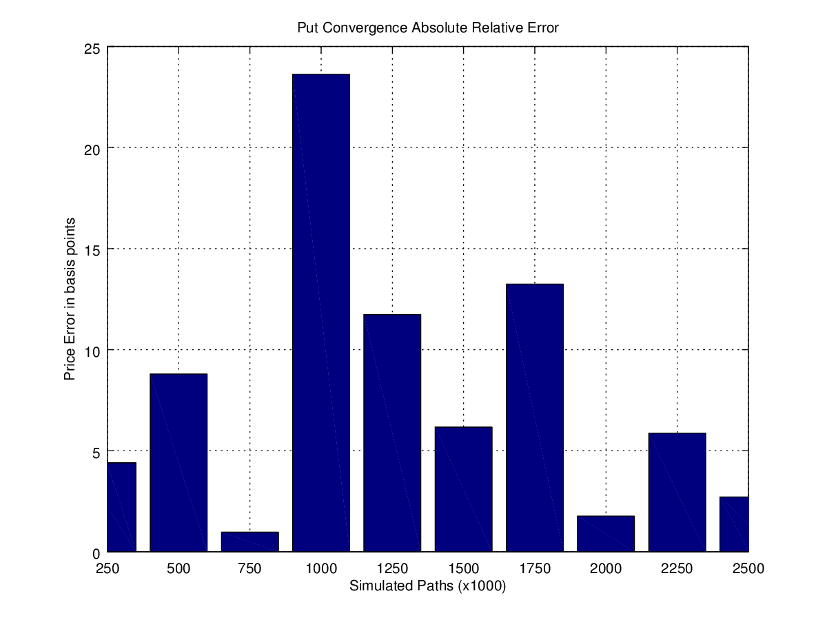
On our development machine the code runs very fast (couple of seconds). That makes it feasible to really experiment with these kinds of simulations. In practical cases where simulation needs to be done multiple times, for example when calibrating a Monte Carlo model, this is a big advantage of using Octave. As a showcase of the kind of output that we normally get please refer to the two series of 3 plots below for the call and put options. The first plot shows the convergence to the closed-form price as the number of scenarios increases in terms of the option price. The second plot zooms in on the errors as the difference between the theoretical price and the simulated price. Finally, the third plot shows the relative error between theoretical and simulated option prices in basis points as absolute number. The number as absolute so it's easier to see convergence.

Call Option

 

 

Put Option

 

 

 

Code Listing

Main Script

% option simulation script
clear; close all;

%constants
TOLERENCE = 1e-12;

% C: call price
% P: put price
% S: stock price at time 0
% X:  strike price
% r: risk-free interest rate
% sigma: volatility of the stock price measured as annual standard deviation
% days: numbers of days remaining in the option contract, this will be converted into unit of years.
% Black-Scholes formula:
%  C = S N(d1) - Xe-rt N(d2)
%  P = Xe-rt N(-d2) - S N(-d1)

T = 0.25
r = 0.02;
S = 95
X = 100;
sigma = 1.21;

% Analytical value
 [C, P]= blackScholes(S,X,r,sigma,T)
 
% put-call parity
% https://en.wikipedia.org/wiki/Put%E2%80%93call_parity
"Check put call parity" 
(C-P) - (S - X * exp(-r * T)) < TOLERENCE


% simulation random walk

n = 2.5e6;
step = 2.5e5;
mu = r;
x = transpose([step:step:n]);
C_mc =zeros(size(x));
P_mc =zeros(size(x));

for i = 1:n/step
  rand('seed', i * n * pi);
  W = randn(i * step,1); 
 
  S_T = S * exp((mu-sigma*sigma*0.5)*T+sigma*sqrt(T)*W);
  C_mc(i) = mean(max(S_T - X, 0))*exp(-r*T);
  P_mc(i) = mean(max(X - S_T, 0))*exp(-r*T);
end

scaler = 1000;
h=figure(1);
stairs(x/scaler,[C_mc, repmat(C, size(x))]);
title('Call Convergence');
xlabel('Simulated Paths');
ylabel('Price');
grid on;
xlim([step/scaler, n/scaler]);
defaultSavePlot(h, "comvergence call.png");

h=figure(2);
bar(x/scaler,[C_mc - repmat(C, size(x))]);
title('Call Convergence Absolute Error');
xlabel('Simulated Paths (x10000)');
ylabel('Price Error');
grid on;
xlim([step/scaler, n/scaler]);
defaultSavePlot(h, "error call.png");

h=figure(3);
bar(x/scaler,[abs(C_mc ./ repmat(C, size(x)) - ones(size(x))) * 10000]);
title('Call Convergence Absolute Relative Error in basis points');
xlabel('Simulated Paths (x1000)');
ylabel('Price Error');
grid on;
xlim([step/scaler, n/scaler]);
defaultSavePlot(h, "relative absolute error call.png");

h=figure(4);
stairs(x/scaler,[P_mc, repmat(P, size(x))]);
title('Put Convergence');
xlabel('Simulated Paths');
ylabel('Price');
grid on;
xlim([step/scaler, n/scaler]);
defaultSavePlot(h, "comvergence put.png");

h=figure(5);
bar(x/scaler,[P_mc - repmat(P, size(x))]);
title('Put Convergence Absolute Error');
xlabel('Simulated Paths (x1000)');
ylabel('Price Error');
grid on;
xlim([step/scaler, n/scaler]);
defaultSavePlot(h, "error put.png");

h=figure(6);
bar(x/scaler,[abs(P_mc ./ repmat(P, size(x)) - ones(size(x))) * 10000]);
title('Put Convergence Absolute Relative Error');
xlabel('Simulated Paths (x1000)');
ylabel('Price Error in basis points');
grid on;
xlim([step/scaler, n/scaler]);
defaultSavePlot(h, "relative absolute error put.png");

BackScholes

function [C, P]= blackScholes(S,X,r,sigma,T)
    d1 = (log(S/X) + (r + 0.5*sigma^2)*T)/(sigma*sqrt(T));
    d2 = d1 - sigma*sqrt(T);
    N1 = 0.5*(1+erf(d1/sqrt(2)));
    N2 = 0.5*(1+erf(d2/sqrt(2)));
    C = S*N1-X*exp(-r*T)*N2;

    N1 = 0.5*(1+erf(-d1/sqrt(2)));
    N2 = 0.5*(1+erf(-d2/sqrt(2)));
    P = X*exp(-r*T)*N2 - S*N1;
end

 

Default Save Plot

function x = defaultSavePlot(plotHandle, name)
  W = 8; H = 6;
  set(plotHandle,'PaperUnits','inches');
  set(plotHandle,'PaperOrientation','portrait');
  set(plotHandle,'PaperSize',[H,W]);
  set(plotHandle,'PaperPosition',[0,0,W,H]);
  print(plotHandle,'-dpng','-color', name);
end