In this blog the basics of generating and saving plots to file using Octave will be demonstrated. We are going to make plots and do some basic data analysis on the Deutsche Bank stock prices. Deutsche has been under pressure these last days, which rose our curiosity.
Deutsche Bank shares collapsed by nearly 7% taking it close to a 30-year low on Thursday evening following reports that hedge funds were pulling assets from it amid suggestions the German government may be forced to bail it out.
Deutsche Bank's share price approaches 30-year low -The Guardian
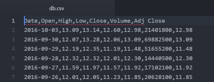
Data
For this analysis we took data from Yahoo Finance from 4 october 2010 to 3 october 2016.
The tricky bit is reading the date field. This requires reading the date as 3 separate fields by splitting them using the ''-" as a separator sign. To make the plots more intuitive we also reorder the data so the oldest date is the first in the list using "flip". This will make the plots read from left to right, which seems the more logical thing to do. Finally, we compute the returns so they can be analyzed.
% Read data from file
fidi = fopen('db.csv');
data = textscan(fidi, '%d %d %d %f %f %f %f %d %f', ...
    'Delimiter',', -','HeaderLines',1);

% Date	Open	High	Low	Close	Volume	Adj Close
price = flip(data(1,9){1});
open = flip(data(1,4){1});
high = flip(data(1,5){1});
low = flip(data(1,6){1});

timeline = flip(datenum(double(data(1,1){1}),
                        double(data(1,2){1}),
                        double(data(1,3){1})
                ));

volume = flip(data(1,8){1});

delta = diff(price);
nPrice = length(price);
returns = delta ./ price(2:nPrice);
Stock Price & Volume
Visualization of the data is straightforward when the data has been imported. To create plots of the price and volume we use:
h=figure(1);
plot(timeline, price, timeline,low, timeline,high,timeline,open);
title('Stock Price Evolution');
xlabel('Date');
ylabel('Price');
datetick('x', 'QQ-YYYY');
L=legend('Close', 'Low', 'High', 'Open');
xlim([timeline(1), timeline(nPrice)]);
grid on;
defaultSavePlot(h, "price.png");

h=figure(2);
stem(timeline, volume)
title('Daily Traded Volume');
datetick('x', 'QQ-YYYY');
grid on;
xlim([timeline(1), timeline(nPrice)]);
xlabel('Date');
defaultSavePlot(h, "volume.png");
With the defaultSavePlot function to set some basic parameters for the plots.
function x = defaultSavePlot(plotHandle, name)
  W = 8; H = 6;
  set(plotHandle,'PaperUnits','inches');
  set(plotHandle,'PaperOrientation','portrait');
  set(plotHandle,'PaperSize',[H,W]);
  set(plotHandle,'PaperPosition',[0,0,W,H]);
  print(plotHandle,'-dpng','-color', name);
end
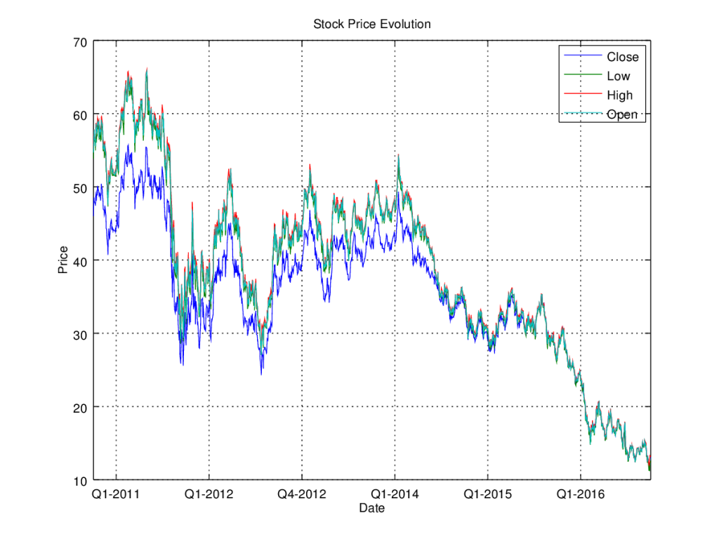
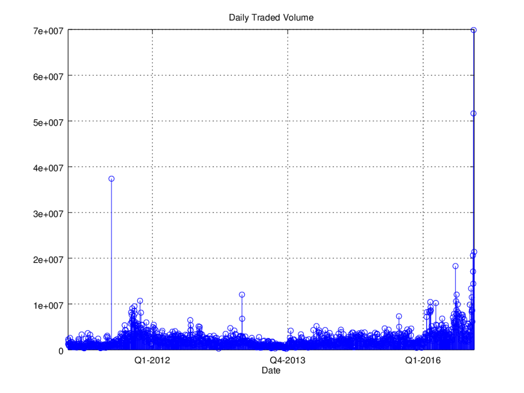
We can clearly see there is a correlation between large price moves (returns) and volumes. This is no surprise as one would expect to see large price changes under large volume for a liquid asset, like Deutsche Bank, as many investors buy or sell the asset.
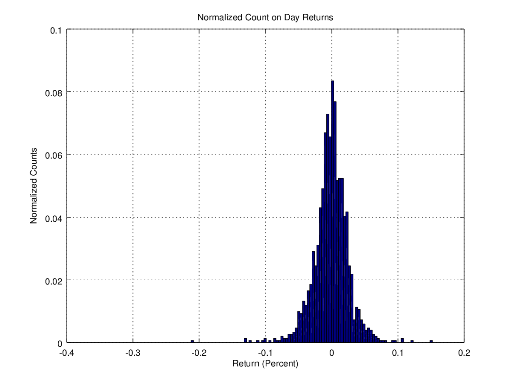
Returns
Next we visualize the returns in a histogram using:
h=figure(3);
hist(returns, 100, 1.0);
title('Normalized Count on Day Returns');
xlabel('Return (Percent)');
ylabel('Normalized Counts');
grid on;
defaultSavePlot(h, "returns.png");
Multiple Plots
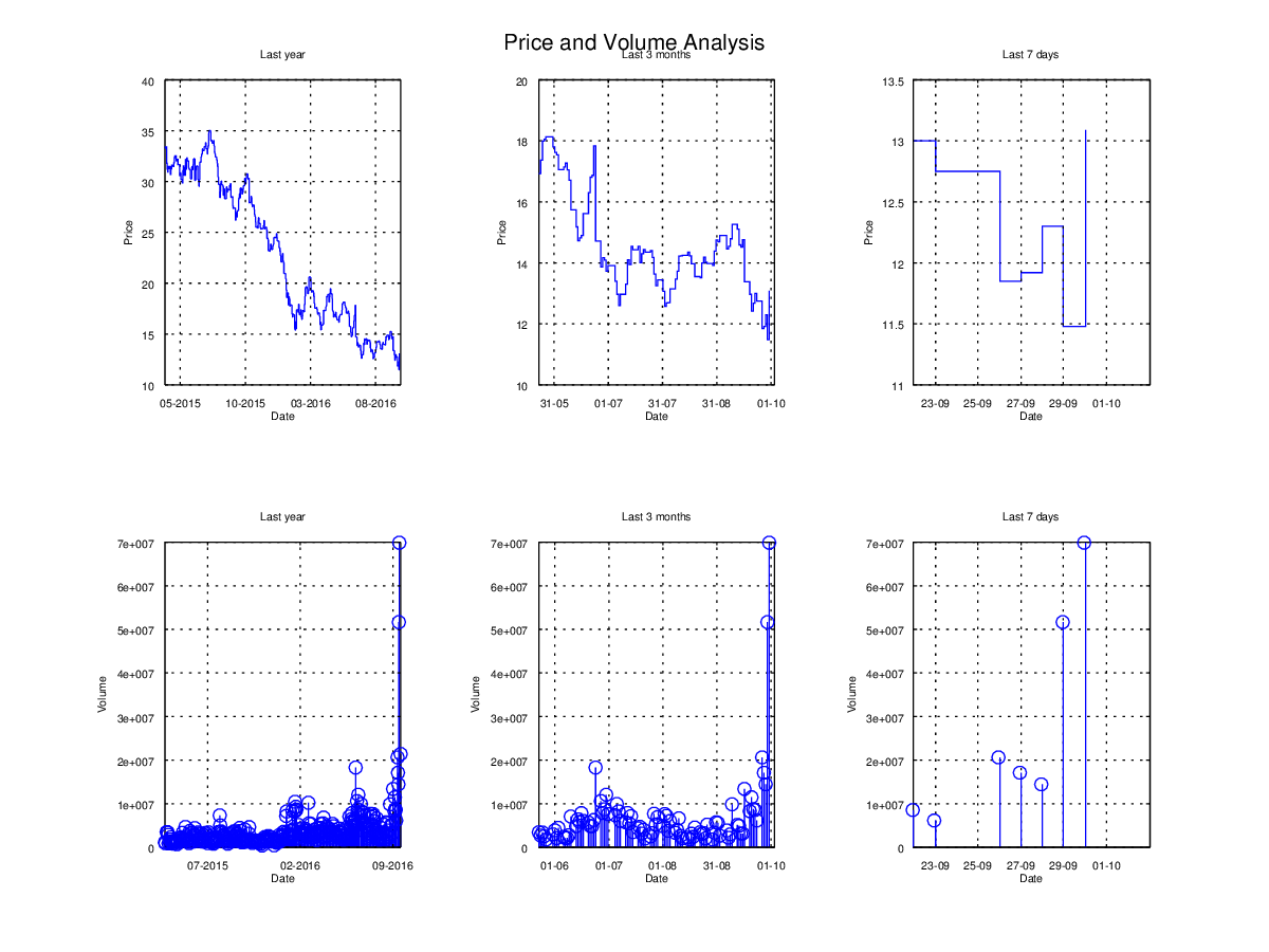
To see what Octave can do in terms of graphics we create an overview of the price and volumes data for 1 year, 3 months and one week horizon. The price subplots are created using “stairs” plots to underline the fact that the data is daily and thus not continuous.
h=figure(5);
subplot(2,3,3)
stairs(timeline(nPrice-7:nPrice-1), price(nPrice-7:nPrice-1));
title('Last 7 days', "FontSize", FONT_SIZE);
xlabel('Date', "FontSize", FONT_SIZE);
ylabel('Price', "FontSize", FONT_SIZE);
datetick('x', 'DD-mm');
xlim([timeline(nPrice-7), timeline(nPrice)]);
set(gca, "FontSize", FONT_SIZE);
grid on;

subplot(2,3,6)
stem(timeline(nPrice-7:nPrice-1), volume(nPrice-7:nPrice-1));
title("Last 7 days", "FontSize", FONT_SIZE);
xlabel('Date', "FontSize", FONT_SIZE);
ylabel('Volume', "FontSize", FONT_SIZE);
datetick('x', 'DD-mm');
xlim([timeline(nPrice-7), timeline(nPrice)]);
set(gca, "FontSize", FONT_SIZE);
grid on;

subplot(2,3,2)
stairs(timeline(nPrice-92:nPrice-1), price(nPrice-92:nPrice-1));
title('Last 3 months', "FontSize", FONT_SIZE);
xlabel('Date', "FontSize", FONT_SIZE);
ylabel('Price', "FontSize", FONT_SIZE);
datetick('x', 'DD-mm');
xlim([timeline(nPrice-92), timeline(nPrice)]);
set(gca, "FontSize", FONT_SIZE);
grid on;

subplot(2,3,5)
stem(timeline(nPrice-92:nPrice-1), volume(nPrice-92:nPrice-1));
title("Last 3 months", "FontSize", FONT_SIZE);
xlabel('Date', "FontSize", FONT_SIZE);
ylabel('Volume', "FontSize", FONT_SIZE);
datetick('x', 'DD-mm');
xlim([timeline(nPrice-92), timeline(nPrice)]);
set(gca, "FontSize", FONT_SIZE);
grid on;

subplot(2,3,1)
stairs(timeline(nPrice-365:nPrice-1), price(nPrice-365:nPrice-1));
title("Last year", "FontSize", FONT_SIZE);
xlabel('Date', "FontSize", FONT_SIZE);
ylabel('Price', "FontSize", FONT_SIZE);
datetick('x', 'mm-YYYY');
xlim([timeline(nPrice-365), timeline(nPrice)]);
set(gca, "FontSize", FONT_SIZE);
grid on;

subplot(2,3,4)
stem(timeline(nPrice-365:nPrice), volume(nPrice-365:nPrice));
title("Last year", "FontSize", FONT_SIZE);
xlabel('Date', "FontSize", FONT_SIZE);
ylabel('Volume', "FontSize", FONT_SIZE);
datetick('x', 'mm-YYYY');
xlim([timeline(nPrice-365), timeline(nPrice)]);
grid on;
set(gca, "FontSize", FONT_SIZE);
ax=axes('Units','Normal','Position',[.075 .075 .85 .85],'Visible','off');
set(get(ax,'Title'),'Visible','on')
title("Price and Volume Analysis");
defaultSavePlot(h, "analysis.png")
References
Engineering Liberty - Blog on creating and saving plots in Octave :
https://engineeringliberty.wordpress.com/2011/10/07/making-great-plots-in-octave-and-matlab-too/
John F. McGowan - Plotting and Graphics in Octave
http://math-blog.com/plotting-and-graphics-in-octave/
Code .M
Complete files in .Zip
Here is a link to the m-files in a zip : data-analysis
Analysis.m
clear;clc;close all;

% plot settings
FONT_SIZE = 5;


% Read data from file
fidi = fopen('db.csv');
data = textscan(fidi, '%d %d %d %f %f %f %f %d %f', ...
    'Delimiter',', -','HeaderLines',1);

% Date	Open	High	Low	Close	Volume	Adj Close
price = flip(data(1,9){1});
open = flip(data(1,4){1});
high = flip(data(1,5){1});
low = flip(data(1,6){1});

timeline = flip(datenum(double(data(1,1){1}),
                        double(data(1,2){1}),
                        double(data(1,3){1})
                ));

volume = flip(data(1,8){1});

delta = diff(price);
nPrice = length(price);
returns = delta ./ price(2:nPrice);

h=figure(1);
plot(timeline, price, timeline,low, timeline,high,timeline,open);
title('Stock Price Evolution');
xlabel('Date');
ylabel('Price');
datetick('x', 'QQ-YYYY');
L=legend('Close', 'Low', 'High', 'Open');
xlim([timeline(1), timeline(nPrice)]);
grid on;
defaultSavePlot(h, "price.png");

h=figure(2);
stem(timeline, volume)
title('Daily Traded Volume');
datetick('x', 'QQ-YYYY');
grid on;
xlim([timeline(1), timeline(nPrice)]);
xlabel('Date');
defaultSavePlot(h, "volume.png");

h=figure(3);
hist(returns, 100, 1.0);
title('Normalized Count on Day Returns');
xlabel('Return (Percent)');
ylabel('Normalized Counts');
grid on;
defaultSavePlot(h, "returns.png");

h=figure(4);
stairs(timeline,price);
title('Evolution of Price');
xlabel('Date');
ylabel('Price');
datetick('x', 'QQ-YYYY');
xlim([timeline(1), timeline(nPrice)]);
grid on;
defaultSavePlot(h, "price_stairs.png");

h=figure(5);
subplot(2,3,3)
stairs(timeline(nPrice-7:nPrice-1), price(nPrice-7:nPrice-1));
title('Last 7 days', "FontSize", FONT_SIZE);
xlabel('Date', "FontSize", FONT_SIZE);
ylabel('Price', "FontSize", FONT_SIZE);
datetick('x', 'DD-mm');
xlim([timeline(nPrice-7), timeline(nPrice)]);
set(gca, "FontSize", FONT_SIZE);
grid on;

subplot(2,3,6)
stem(timeline(nPrice-7:nPrice-1), volume(nPrice-7:nPrice-1));
title("Last 7 days", "FontSize", FONT_SIZE);
xlabel('Date', "FontSize", FONT_SIZE);
ylabel('Volume', "FontSize", FONT_SIZE);
datetick('x', 'DD-mm');
xlim([timeline(nPrice-7), timeline(nPrice)]);
set(gca, "FontSize", FONT_SIZE);
grid on;

subplot(2,3,2)
stairs(timeline(nPrice-92:nPrice-1), price(nPrice-92:nPrice-1));
title('Last 3 months', "FontSize", FONT_SIZE);
xlabel('Date', "FontSize", FONT_SIZE);
ylabel('Price', "FontSize", FONT_SIZE);
datetick('x', 'DD-mm');
xlim([timeline(nPrice-92), timeline(nPrice)]);
set(gca, "FontSize", FONT_SIZE);
grid on;

subplot(2,3,5)
stem(timeline(nPrice-92:nPrice-1), volume(nPrice-92:nPrice-1));
title("Last 3 months", "FontSize", FONT_SIZE);
xlabel('Date', "FontSize", FONT_SIZE);
ylabel('Volume', "FontSize", FONT_SIZE);
datetick('x', 'DD-mm');
xlim([timeline(nPrice-92), timeline(nPrice)]);
set(gca, "FontSize", FONT_SIZE);
grid on;

subplot(2,3,1)
stairs(timeline(nPrice-365:nPrice-1), price(nPrice-365:nPrice-1));
title("Last year", "FontSize", FONT_SIZE);
xlabel('Date', "FontSize", FONT_SIZE);
ylabel('Price', "FontSize", FONT_SIZE);
datetick('x', 'mm-YYYY');
xlim([timeline(nPrice-365), timeline(nPrice)]);
set(gca, "FontSize", FONT_SIZE);
grid on;

subplot(2,3,4)
stem(timeline(nPrice-365:nPrice), volume(nPrice-365:nPrice));
title("Last year", "FontSize", FONT_SIZE);
xlabel('Date', "FontSize", FONT_SIZE);
ylabel('Volume', "FontSize", FONT_SIZE);
datetick('x', 'mm-YYYY');
xlim([timeline(nPrice-365), timeline(nPrice)]);
grid on;
set(gca, "FontSize", FONT_SIZE);
ax=axes('Units','Normal','Position',[.075 .075 .85 .85],'Visible','off');
set(get(ax,'Title'),'Visible','on')
title("Price and Volume Analysis");
defaultSavePlot(h, "analysis.png")
max_return = max(returns);
max_return_info = dayInfo(max_return, returns, timeline, delta, price, volume)
min_return = min(returns);
min_return_info = dayInfo(min_return, returns, timeline, delta, price, volume)
mean_return = mean(returns)
std_return = std(returns)
DayInfo.m
function x = dayInfo(returnToFind, returns, timeline, delta, price, volume)
%
% Finds the return in the list and returns details of day
% Use to find max, min ect. day info
  x =struct(
      "return", returnToFind,
      "date", datestr(timeline(find(returns==returnToFind))),
      "delta", delta(find(returns==returnToFind)),
      "price", price(find(returns==returnToFind)),
      "volume", volume(find(returns==returnToFind))
    );
end
DefaultSavePlot.m
function x = defaultSavePlot(plotHandle, name)
  W = 8; H = 6;
  set(plotHandle,'PaperUnits','inches');
  set(plotHandle,'PaperOrientation','portrait');
  set(plotHandle,'PaperSize',[H,W]);
  set(plotHandle,'PaperPosition',[0,0,W,H]);
  print(plotHandle,'-dpng','-color', name);
end