Introduction
The course I am teaching considers option valuation methodologies, in particular the Black Scholes and binomial tree. There are many steps needed to derive these models. In preparation for teaching the next class on the binomial tree model, I thought it would be useful to share my notes.

About the option market
Options are financial derivatives used to transfer volatility risk from one party to the next. Starting back in the Roman Empire where contracts were traded on olives. Options have been around ever since, but their value was unclear. Traders would quote prices based on intuition rather than reason making options obscure instruments.
In 1900, Bachelier published his thesis and in doing so pioneered modern financial engineering. Options now entered the academic world, becoming an interesting research topic. Options didn’t shed their obscure and academic image until in 1973 the Chicago Board Options Exchange (CBOE) opened for business as the first option exchange. On the first day of trading, April 26, 911 contracts traded on 16 underlying stocks.Cox and Rubinstein commented on this monumental day for option trading;

Although options have been traded for centuries, they were, until recently, relatively obscure and unimportant financial instruments. Options markets were fragmented , and transactions were both costly and difficult to arrange. All this changed when in 1973 with the creation of the Chicago Board Options Exchange, the first registered securities exchange for the purpose of trading options.
Cox (1985)

The CBOE was important in offering standardised contracts for trading, first only for call options and later for both call and put options. In 1973, Black and Scholes published their now famous paper with the option pricing formula. This formula changed the market, but wasn’t compete at the time. It only dealt with European style options and did not consider dividend. Cox and Rubinstein’s binomial model solved both these problems in 1979. Currently the Black-Scholes model has been extended and widely accepted. Making the binomial model less relevant on trading floors.

Because the binomial model is easier to explain and understand, it is a good model to start with when studying option valuation. We used this model to demonstrate option pricing to the students last week.

Model
Let’s start with a small model and build outwards from there. Consider an economy with only one asset . The economy only has two possible future states: a positive scenario where the value of the asset increases and a negative scenario where it decreases.
A new derivative (V) is introduced into the economy the value of which is dependent on the asset (S), the underlying. We construct a portfolio of one derivative and a to be determined number (∆) of underlying assets:

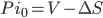  (1)

The value of the portfolio can have only two future values, based on the two future states of the economy. If the asset increases in value it will do so by a factor u. In this case the value of the portfolio becomes:

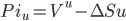    (2)

If the the value of the asset decreases it does do by a factor of d. The value of the resulting portfolio is given by:

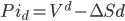    (3)

Assume that the probability of the asset increasing in value equals p. This implies that the probability of the asset decreasing in value is (1-p). Using these probabilities, the present value of the future portfolios can be computed as follows:

    (4)

In the equation above we discount using a continuous interest rate (r) during the lifetime (T) of the derivative. The equation computes the expected value of the option using real world chances as estimated by the market.
To make the portfolio risk neutral we have to choose ∆ so that one is indifferent between the future value of the portfolio, considering both the asset value increasing and decreasing. To find the value of ∆ that does that, equations 2 and 3 must be equal.

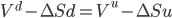   (5)

Solving this equation for ∆ gives:

   (6)

If ∆ is chosen, as in equation 6, it is without consequence in which state the economy ends (u or d). Conclusion: there is no risk. The value of the portfolio is no longer influenced by the value of the asset and is known a priori. Now the outcome is fixed we no longer need the probabilities of the up and down states of the economy, we can simply discount a known cash flow. Here the scenario with increasing asset value is used ¹:

   (7)

The value of derivative V can now be computed by substituting equation 6 for ∆ in equation 7, leaving us with:

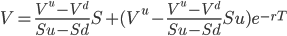    (8)

The formula can be rewritten to find new probability q, the probability without risk.

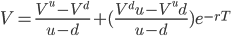    (9)

Grouping the terms gives:

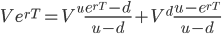  (10)

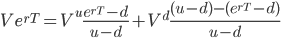
Now we can define the risk neutral probability q as:

   (11)

Reorganising equation 10 to accommodate q:

  (12)

Substituting equations 11 in 12 yields the value of the derivative using risk neutral probabilities:

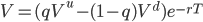   (13)

The value of the portfolio now becomes:

    (14)

We have seen two ways of computing values, one based on real world probabilities (equation 4) and one based on risk neutral probabilities (equation 14). The risk neutral probabilities have no link with the real world.
The equations are different yielding different results, which one is correct? Let’s try and find out by example.

Worked example; real world versus risk neutral probabilities
Setting up a risk neutral portfolio has led us to risk neutral probabilities (q) to compute its value. This probability is different from the real world probability (p). In this example the difference between the two will be illustrated.
Example
Consider a portfolio containing a call option with a strike of 21 on a stock with a current value of 20. The market agrees that there is a 70% chance of the stock price going up to 22 (u=1.1) at option expiration. There is a 30% chance of the stock price dropping to 18 (d=0.9). To make matters simple consider the interest 0% (r=0.0, hence no discounting required).
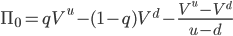
Given this example it follows that there is a 70% chance on the call option payoff being 1 and a 30% chance of the option being worthless at expiration. The expected value of the call option using real world probabilities is:

Using the risk neutral probabilities we find:

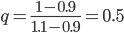
Using equation 13 the value of the option is:

As expected the two methods yield different results. Assuming you find a buyer for a call option for 70 cents.What should you do?
-Sell the option and receive 70 cents cash.
-Borrow 430 cents.
-Buy 0.25 stock for 500 cents.

Now there are two possibilities. The stock price ends at 22 or 18.

If it ends at 22:
-Payout 100 cents to the owner of the call option.
-Sell the 0.25 stock for 550 cents.
-Pay back the loan of 500 cents.
-Net result +70-100+550-500=20 cents profit.

What happens if the price drops to 18?
-No payout to the call option owner required.
-Sell 0.25 stock for 450 cents.
-Pay back loan 500 cents
-Net result +70-0+450-500=20 cents profit.

We have created a money machine! In both cases we make 20 cents profit with out taking any risk. If this would happen in real life, sooner or later somebody would spoil the game by offering the option for 69 cents. If there is someone that will settle for only 19 cents profit margin, chances are there will also be someone who will settle for 18. In the end all margin will be gone. In the end the contract will trade only for its fair price of 50 cents. It is no coincidence that this is the risk neutral price we computed.

Notes
The binomial tree model can be generalised by creating a tree of binomial models. Maybe in the case of the example it would look something like this:

This makes the model richer and easier to fit on real market data. There are many good books how explain this in details, for example Hull(2008) and Cox(1985). This kind of detail is outside of the scope of this note. If you want to get a feel for the model consider downloading this model [http://demonstrations.wolfram.com/BinomialTree/].

Summary
In this noted it was show that real world probabilities don’t yield the correct price, but risk neutral probabilities do. This conclusion was reached by considering the binomial model first introduced by Cox and Rubenstein.
In this note uses more steps to derive the required equations than most papers, since its primary goal is to serve as an introduction to those new to financial mathematics in a classroom setting.

References
Black F., Scholes M. (1973), The Pricing of Options and Corporate Liabilities, Journal of Political Economy 81 (3): 637–654
Cox J. C., Rubinstein M. (1985), Option Markets, Prentice Hall
Hull, J. C. (2008), Options, Futures, and Other Derivatives (7th Edition), Prentice Hall
Bachelier, L. (1900), Théorie de la spéculation, 1900, Gauthier-Villars, 70 pp.

Web recoures
Chicago Board Options Exchange, http://www.cboe.com/aboutcboe/History.aspx
OptionTradingPenia, http://www.optiontradingpedia.com/history_of_options_trading.htm

Originally posted on http://financialagile.uglyduckling.nl/finance/option-pricing-with-the-binomial-model/