Introduction
Black, Scholes and Merton’s famous option price formula wasn’t a new discovery, as shown in the next section. The formula was well know at the time and widely used in the option market. Often it is noted that option trading took off after the publication of the Black-Scholes formula, but this simply is not true... however, the reverse is. In 1973 the Chicago Board Options Exchange (CBOE) opened for business as the first option exchange in the world, making options widely available. This and the introduction of handheld calculators, to do the necessary computations for Black and Scholes, made the formula a success. The formula may not have been a break through, but the way it was derived certainly was. Using the risk free portfolio was the step that made the known formula acceptable to academia. The derivation of the formula is the topic of this note based on research I did for a class on derivatives.

Before Black & Scholes

Options have been around for a long time, as far back as the days of the Roman empire. Back then there was no Black-Scholes formula to guide price setting. Before the first world war options were traded in Amsterdam, Paris, London and New York. There were even firms specialising in arbitraging the markets. This involved telegrams and shipping actual paper stocks! It has been documented that the market already knew about put-call parity. If the parity is known, price setting becomes an inventory exercise, since put can be changed in calls and vice versa. There were specialists called converters who did only this.
If there was no inventory at hand, a market maker knew that they should hedge their position using the underlying asset. Nelson describes this concept already in 1904. Later the concept is generalised and extended by Thorp from ‘at the money hedge’ to ‘off the money hedging’, essentially formulating the concept of ∆-hedging.

Thorp went on to make a small fortune by discovering risk neutral probabilities and putting the concept to practice in the Las Vegas casinos. He also went on to discover the formula now know as the Black-Scholes equation. Thorp formulated the equation, but didn’t have a derivation at first. It was Black and Scholes who added the dynamic hedging concept used to make a portfolio of a derivative and its underlying asset risk free, allowing for the derivation of the equation. Black and Scholes cemented knowledge that had been around in practice for some time into the academic world using the the concept of the replicating portfolio. A concept considering that the value of a derivative at payoff would be perfectly replicated by a continuously rebalanced portfolio of the underlying and the risk free asset. This implies that the option value is equal to the portfolio value, with an equivalence between the continuous rebalancing and delta hedging your position.

Derivation of the Equation
The history of mathematical finance starts with small particles randomly moving in a fluid named after the botanist, Robert Brown, who first observed them. Later Bachelier (1900), Einstein (1905) and finally Wiener (1923) developed a rigorous theory and the mathematics to describe Brownian Motion. The resulting theory is essential for the derivation of the Black and Scholes formula, which uses Brownian Motion to model asset prices as stochastic differential equations. To work with these equations we need Ito calculus. Ito (1951) showed how given a stochastic differential equation for some independent random variable, one can derive the stochastic differential equation of a function of that variable.

OK, time to start this derivation... The foundation of the derivation is the observation that perfect correlation exists between the asset (S) and its derivative (V (S, T )). This correlation will be exploited to acquire the required result. Consider the portfolio Π of one long option position and short a quantity ∆ of the underlying asset:

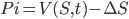 [1]

Assume that the asset price evolves according to the geometric Brownian motion with expected asset return of µ and volatility σ:

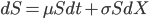[2]

Where dX denotes the stochastic Brownian motion, i.e. a random walk build up by a series of  independent increments drawn form the standard normal distribution. We consider how the portfolio responds to price changes in the underlying.

 [3]

Since the derivative is dependent on the asset (represented by a stochastic differential equation) we can use Ito’s lemma to find an expression dV.

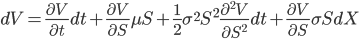  [4]

Now the the change in the value in the portfolio can be written as:

 [5]

Wouldn’t it be nice if we could get rid of all these stochastic terms? That would make dealing with the equation much easier (equivalent to previous note on the binomial tree). Can we find a choice of ∆ that eliminates all the dX terms? Yes, choose:

  [6]

Something amazing happens using this choice of ∆, the μ-term also disappears! Implying that
we no longer face the difficult task of coming up with a number for stock return (μ). The solution is independent of individual return expectations. More importantly choosing ∆ we eliminate risk, i.e.  hedge our position. We are left with a risk free portfolio, since the equation no longer contains a dX term.

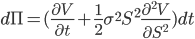  [7]

Since our portfolio is completely free of risk it can only grow at the same rate as a (default free) bank account. A portfolio invested in a bank account, paying the risk free rate r, is defined by :

  [8]

Since the bank account is the only other risk free portfolio in the market and it is considered that there is no arbitrage, the two must be equal.

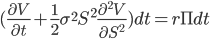  [9]

After substituting equation [8] into [9] and re-arranging the result the famous Black and Scholes partial differential equation can be found:

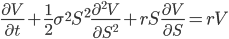 [10]

This is all that will be covered here. If you want to retrieve the option pricing formula you need to choose the following payoff functions for respectively the call and put option with strike K:

V=Max(S-K,0)
V=Max(K-S,0)

Substituting these payoffs and solving the equation will yield the required result. Since solving this problem, known in physics as the heat equation, is out side the scope of the class it is not considered here.

Assumption and their problems
Assumption 1: Dynamic hedging can’t be done
If we would want to implement the formula, it requires us to constantly update the ∆ so we are hedged and the risk free portfolio assumption holds. What does this mean? Hedge at the end of every day? But what if a major event happens in the middle of the day? We would be too late. Being too late will still be a problem if we rebalance the hedge every hour, or minute. Although we would reduce the chance of being to late the more often we rebalance. To make this assumption hold we would have to continuously rebalance the hedge, which simple isn’t feasible in practice.

Assumption 2: Constant volatility
The goal of an option is to transfer volatility (risk) from one party to the next. Even though its the most common use, the formula we derived isn’t limited to options. For such a key parameter it is strange to consider it constant for the lifetime of the option. Perhaps volatility will be constant for the short term, but it most certainly will not for the long term. This is the single biggest problem with the formula.

Assumption 3: Efficient markets
The asset price is modeled by a Brownian motion, which implies that we consider it to be truly random. This means nobody can consistently predict if assets will go up or down given the known price history.

Assumption 4: No dividends
In the model we don’t consider dividends. In the current economic crisis you would almost forget, but real assets pay dividends. This is not a major short coming in the model and has been remedied long ago.

Assumption 5: Risk free rate is constant
In practice this simply doesn’t exist. Since the hedge will need adjusting during the life of the option we will need to borrow or deposit money. There is no way of knowing at which time and rate this will occur, but certainly the interest rate will fluctuate. Besides this issue there is the problem of there being no such thing as a risk free rate, there is always a chance the counter party will default how ever remote it may be.

Assumption 6: Only works for european options
Most exchange traded options are american, making this an issue.

Assumption 7: Log normally distributed returns
The BackScholes model implies asset returns being log normally distributed. Empirical evidence shows that this simply isn’t the case. Extreme scenarios happen much more often than the distribution accounts for. Pick a time series of any major index to confirm this,if you like.

Assumption 8: No transaction costs
The model doesn’t account for any cost in trading.

Assumption 9: Liquidity
This is a major constraint, which is often not understood. During extreme events, markets just don’t work. The future market closes in case of extreme price fluctuation (limit up or down). Market makers might not want to quote “realistic” prices for options. You might not be able to borrow any more money or assets (to go short). There may be a shortage of the underlying to hedge your position with. What works in theory might not be possible to execute. It is very likely that the delta you find isn’t a nice round number, but something like ∆=12.346. There is no trading 12.346 shares in the market. In extreme (market) situations there might not be any trading at all, for example during the 9/11 aftermath markets were closed.

Conclusion
In this note is was shown that the derivation of the Black Scholes differential equation is based on an important concept of creating a risk free portfolio by hedging the risk. Although both the practical relevance of the derivation and assumptions can be questioned it has proven to be very important from a theoretical point of view. The Black-Scholes formula is at least accepted to the extent that often prices of options are quoted in Black-Scholes implied volatility, even though traders likely use more complex models to actually value the options themselves. The sensitivity to market parameters (the so called Greeks) are very important and used around the world to monitor risk.

Reference
Bachelier, L. (1900), Théorie de la spéculation, 1900, Gauthier-Villars, 70 pp.
Black F., Scholes M. (1973), The Pricing of Options and Corporate Liabilities, Journal of Political Economy 81 (3): 637–654
Brown, R. (1827), A brief Account of Microscopical Observations, London
Haug, E., Taleb, N. (2010), Why We Have Never Used the Black-Scholes-Merton Option Pricing Formula (fifth version), working paper
Nelson, S. A. (1904), The A B C of Options and Arbitrage, New York Thorp, E. (1962), Beat the Dealer, Vintage Books
Wiener, N. (1923), Differential space, Journal of Mathematics and Physics, 58 131-74
Wilmott, P. (2007), Frequently ask questions in quantitate finance, Wiley

Internet Resources
Chicago Board Options Exchange, http://www.cboe.com/aboutcboe/History.aspx
http://web.archive.org/web/20150511011038/http://www.capital-flow-analysis.com:80/investment-essays/nobel_gods.html [update 4/4/2016 resource no longer online]
http://en.wikipedia.org/wiki/Black–Scholes
Black Scholes calculator http://www.blobek.com/black-scholes.html

Originally posted on http://financialagile.uglyduckling.nl/finance/option-pricing-with-black-scholes/